Developer Guide

Module Implementation

Fig. 26 and Fig. 27 show schematic representations of the three different aspects of a module, using the StarCatalog and Observatory modules as examples, respectively. Every module has a prototype that defines the module’s standard attributes and methods, including their input/output structure. Prototype implementations also frequently implement common functionality that is reused by all or most implementations of that module type. The various implementations inherit the prototype and add/overload any attributes and methods required for their particular tasks, limited only by the preset input/output scheme for prototype methods. Finally, in the course of running a simulation, an object is generated for each module class selected for that simulation. The generated objects can be used interchangeably in the downstream code, regardless of what implementation they are instances of, due to the strict interface defined in the class prototypes. These objects are always called the generic module type throughout the code (implementation class names are used only when specifying which modules to select for a given simulation).

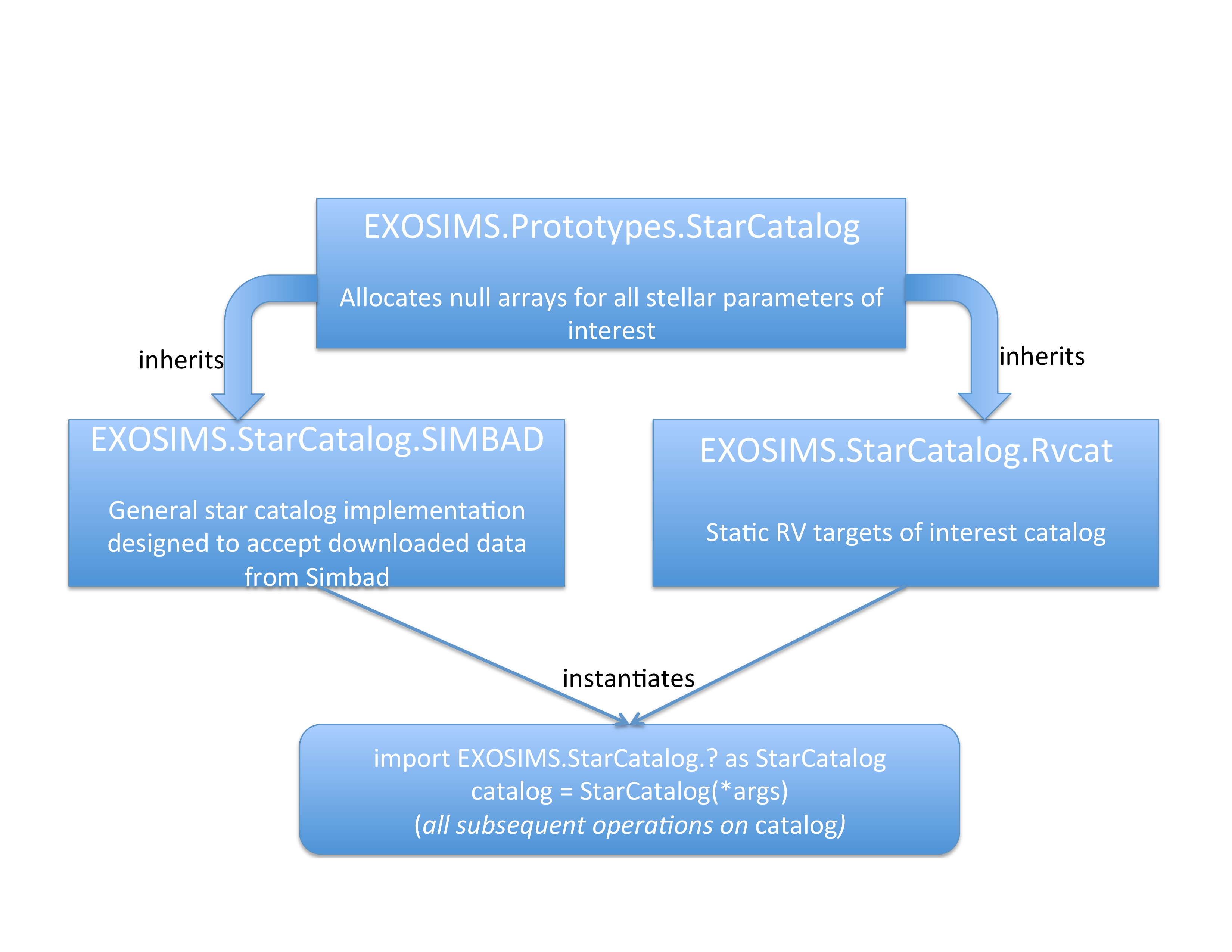
Fig. 26 Schematic of a sample set of implementation for the StarCatalog module. The prototype (top row) is immutable, specifies the input/output structure of the module along with all common functionality, and is inherited by all StarCatalog implementations (middle row). In this case, two different catalog classes are shown: one that reads in data from a SIMBAD catalog dump, and one which contains only information about a subset of known radial velocity targets. The object used at runtime during a simulation (bottom row) is an instance of one of these three classes, is always referred to as StarCatalog in all of the code, and can be used in exactly the same way in the rest of the code due to the common input/output scheme for all required methods.

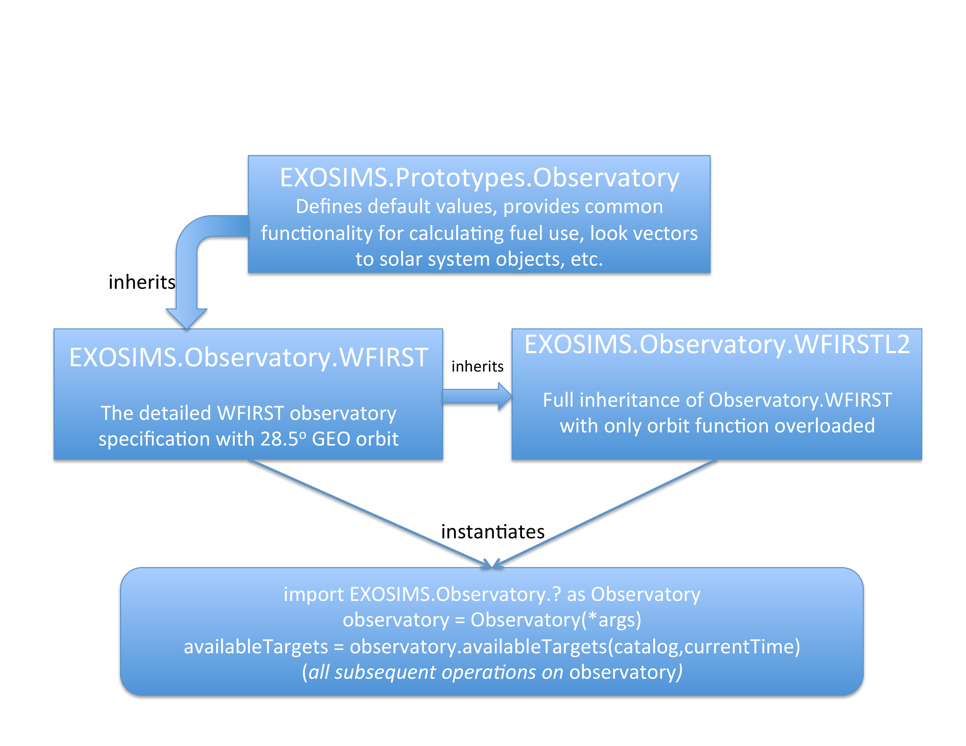
Fig. 27 Schematic of a sample set of implementations for the Observatory module. The prototype (top row) is immutable, specifies the input/output structure of the module along with all common functionality, and is inherited by all Observatory class implementations (middle row). In this case, two different observatory classes are shown that differ only in the definition of the observatory orbit. Therefore, the second implementation inherits the first (rather than directly inheriting the prototype) and overloads only the orbit method. The object used at runtime during a simulation (bottom row) is an instance of one of these classes, is always referred to as Observatory in all of the code, and can be used in exactly the same way in the rest of the code due to the common input/output scheme for all required methods.

For lower level (downstream) modules, the input specification is much more loosely defined than the output specification, as different implementations may draw data from a wide variety of sources. For example, the StarCatalog may be implemented as reading values from a static file on disk, or may represent an active connection to a local or remote database. The output specification for these modules, however, as well as both the input and output for the upstream modules, is entirely fixed so as to allow for generic use of all module objects in the simulation.

Module Inheritance and Initialization

The only requirement on any implemented module is that it inherits the appropriate prototype (either directly or by inheriting another module implementation that inherits the prototype). It is similarly expected (but not required) that the prototype __init__ will be called from the __init__ of the newly implemented class (if the class overloads the __init__ method). Here is an example of the beginning of an OpticalSystem module implementation:

from EXOSIMS.Prototypes.OpticalSystem import OpticalSystem

class ExampleOpticalSystem(OpticalSystem):

    def __init__(self, **specs):

        OpticalSystem.__init__(self, **specs)

        ...

Important

The filename must match the class name for all modules.

Important

If overloading the prototype __init__, the implemented module’s __init__ method must have a keyword argument dictionary input (the **specs argument in the example, above). This must be the last argument to the method. See here for an explanation of the syntax, and see Input Specification for further discussion on this input. Note that the name of the input is arbitrary, but is always **specs in the EXOSIMS prototypes.

Module Type

It is always possible to check whether a module is an instance of a given prototype, for example:

isinstance(obj,EXOSIMS.Prototypes.Observatory.Observatory)

However, it can be tedious to look up all of a given object’s base classes so, for convenience, every prototype will provide a private variable _modtype, which will always return the name of the prototype and should not be overwritten by any module code. Thus, if the above example evaluates as True, obj._modtype will be equal to Observatory.

Callable Attributes

Certain module attributes may be represented in a way that allows them to be parametrized by other values. For example, the instrument throughput and contrast are functions of both the wavelength and the angular separation, and so must be encodable as such in the OpticalSystem. To accommodate this, as well as simpler descriptions where these parameters may be treated as static values, these and other attributes are defined as ‘callable’. This means that they must be set as objects that can be called in the normal Python fashion, i.e., object(arg1,arg2,...).

These objects can be function definitions defined in the code, or imported from other modules. They can be lambda expressions defined inline in the code. Or they can be callable object instances, such as the various scipy interpolants. In cases where the description is just a single value, these attributes can be defined as dummy functions that always return the same value, for example:

def throughput(wavelength,angle):
     return 0.5

or, more simply:

throughput = lambda wavelength,angle: 0.5

Warning

It is important to remember that Python differentiates between how it treats class attributes and methods in inheritance. If a value is originally defined as an attribute (such as a lambda function), then it cannot be overloaded by a method in an inheriting class implementation. So, if a prototype contains a callable value as an attribute, it must be implemented as an attribute in all inheriting implementations that wish to change the value. For this reason, the majority of callable attributes in prototype modules are instead defined as methods to avoid potential overloading issues.

Units

All attributes/variables representing quantities with units are encoded using astropy.units.quantity.Quantity objects. Docstrings will often state the default unit used for quantities, but it is never necessary to assume a unit, other than for inputs (see Input Specification).

Unit Performance Tips

While astropy.units.quantity.Quantity provides crucial type safety and dimensional analysis, computations involving Quantity and Unit objects introduce significant performance overhead. Here are tips for optimizing performance in performance-critical sections:

1. Strip units before computation

   Quantity operations are slower than numpy operations. Convert Quantity objects to numpy arrays or scalar values before entering a loop or performing intensive calculations. Ensure all units are compatible and re-attach units after the computation is complete!

arr1 = np.random.rand(10000) * u.ph / u.s / u.nm / u.m**2 # Star flux
arr2 = np.random.rand(10000) * u.m**2 # Telescope area
arr3 = np.random.rand(10000) * u.nm # Bandwidth
#########
# Slow
#########
x = arr1 * arr2 * arr3
# %timeit x = arr1 * arr2 * arr3
# 27.5 μs ± 720 ns per loop (mean ± std. dev. of 7 runs, 10,000 loops each)
#########
# Fast
#########
x = arr1.value * arr2.value * arr3.value
# %timeit x = arr1.value * arr2.value * arr3.value
# 8.2 μs ± 471 ns per loop (mean ± std. dev. of 7 runs, 100,000 loops each)

2. Precalculate compound units

   Compound units (e.g. u.ph / u.s / u.nm / u.m**2) that are used repeatedly by a module during a simulation should be precalculated in the module’s __init__ method. Even simple units (e.g. 1 / u.s) can add a surprising amount of overhead.

arr = np.random.rand(10000)

########
# Slow
########
x = arr * u.ph / u.s / u.nm / u.m**2
# %timeit x = arr * u.ph / u.s / u.nm / u.m**2
# 38.9 μs ± 860 ns per loop (mean ± std. dev. of 7 runs, 10,000 loops each)

########
# Fast
########
flux_unit = u.ph / u.s / u.nm / u.m**2
x = arr * flux_unit
# %timeit x = arr * flux_unit
# 2.9 μs ± 6.68 ns per loop (mean ± std. dev. of 7 runs, 100,000 loops each)

3. Attach units to arrays with <<

   By default, multiplying a numpy array by a Unit creates a copy of the array. This is often unnecessary and a significant performance hit. Use << to attach units to an array without copying it. For example, the code arr * u.ph / u.s / u.nm / u.m**2 copies the arr array four times and arr << u.ph / u.s / u.nm / u.m**2 does no copying.

arr = np.random.rand(10000)
flux_unit = u.ph / u.s / u.nm / u.m**2
########
# Slow
########
x = arr * flux_unit
# %timeit x = arr * flux_unit
# 3 μs ± 111 ns per loop (mean ± std. dev. of 7 runs, 100,000 loops each)

########
# Fast
########
x = arr << flux_unit
# %timeit x = arr << flux_unit
# 1.31 μs ± 16.2 ns per loop (mean ± std. dev. of 7 runs, 1,000,000 loops each)

4. Use arr.to_value(u.unit) instead of arr.to(u.unit).value

   The Quantity.to_value method, used correctly, is much faster than the .to().value method. to() always creates a copy of the array whereas to_value() returns a view of the original array if the units of arr are already correct. In EXOSIMS we almost always know what the units of a quantity will be, so to_value() provides a lot of flexibility.

flux_unit = u.ph / u.s / u.nm / u.m**2
arr_flux = np.random.rand(10000) << flux_unit

########
# Slow
########
x = arr_flux.to(flux_unit).value
# %timeit x = arr_flux.to(flux_unit).value
# 3.61 μs ± 189 ns per loop (mean ± std. dev. of 7 runs, 100,000 loops each)

########
# Fast
########
x = arr_flux.to_value(flux_unit)
# %timeit x = arr_flux.to_value(flux_unit)
# 285 ns ± 5.99 ns per loop (mean ± std. dev. of 7 runs, 1,000,000 loops each)

5. When specifying units, use the units directly instead of strings

   Astropy allows you do arr.to_value("m/s") but this is slower than arr.to_value(u.m/u.s) because astropy has to parse the string. This becomes especially problematic for compound units where you also lose the option of pre-calculating the unit.

arr = np.random.rand(10000) << u.m / u.s

#########
# Slow
#########
x = arr.to_value("m/s")
# %timeit x = arr.to_value("m/s")
# 18.3 μs ± 314 ns per loop (mean ± std. dev. of 7 runs, 100,000 loops each)

#########
# Fast
#########
x = arr.to_value(u.m/u.s)
# %timeit x = arr.to_value(u.m/u.s)
# 4.06 μs ± 44.2 ns per loop (mean ± std. dev. of 7 runs, 100,000 loops each)

The standard pattern for performance-critical sections is roughly:

1. Precalculate compound units

2. At the start of a function/method convert the inputs to the right units with to_value()

3. Reattach units at the end of the function/method with <<

Here’s a simple count rate calculation before and after optimization:

import astropy.units as u
import numpy as np

# Create arrays for count rate calculations
F_s = np.random.rand(10000) << u.ph / u.s / u.nm / u.m**2 # Star flux
A = 25 * u.m**2 # Telescope area
BW = 100 * u.nm # Bandwidth

 def base_calculation(F_s, A, BW):
     return (F_s * A * BW).to(u.ph / u.s)

 # Precalculate compound units
 count_rate_unit = u.ph / u.s
 flux_unit = u.ph / u.s / u.nm / u.m**2
 m2 = u.m**2
 def optimized_calculation(F_s, A, BW):
     # Convert inputs to the right units
     _F_s = F_s.to_value(flux_unit)
     _A = A.to_value(m2)
     _BW = BW.to_value(u.nm)
     # Multiply and attach units inplace
     return _F_s * _A * _BW << count_rate_unit

#########
# Slow
#########
x = base_calculation(F_s, A, BW)
# %timeit x = base_calculation(F_s, A, BW)
# 42.3 μs ± 1.73 μs per loop (mean ± std. dev. of 7 runs, 10,000 loops each)

#########
# Fast
#########
x = optimized_calculation(F_s, A, BW)
# %timeit x = optimized_calculation(F_s, A, BW)
# 11.4 μs ± 282 ns per loop (mean ± std. dev. of 7 runs, 100,000 loops each)

Coding Conventions

EXOSIMS attempts to follow standard Python coding conventions (PEP-8, etc.) and it is required that all new code be blackened. Descriptive variable and module names are strongly encouraged. Documentation of existing modules follows the Google docstring style, although the NumPy style is acceptable for new contributions. For more details, see Docstrings.

The existing codebase (as it was written by many different contributors) contains a wide variety of naming conventions and naming styles, including lots of CamelCase and mixedCase names. The project PI thinks these look pretty and is firmly unapologetic on this point.

Interface Specification

The docstrings for the prototypes (see Framework) are the interface control documentation (ICD) for EXOSIMS.

Warning

Module implementations overloading a prototype method may not modify the calling syntax to the method. Doing so will almost invariably cause the new module to not function properly within the broader framework and will almost certainly cause unit tests to fail for that implementation.

New implementations must adhere to the interface specification, and should seek to overload as few methods as possible to produce the desired results. Any change in the method declaration in any prototype is considered interface breaking and will result in a software version bump.